File-IO
In the last four sessions we’ve covered most of the basic concepts of programming in Python. However, one important aspect that we have not yet touched on is how to read from and write to files on your computer using Python code. This is a crucial skill for any programmer, as it allows you to avoid manually entering data.
We call the process of reading from and writing to files file input/output (file I/O). In this session, we will explore the basics of file I/O in Python, including how to open, read, write, and close files.
Uploading files to Noteable
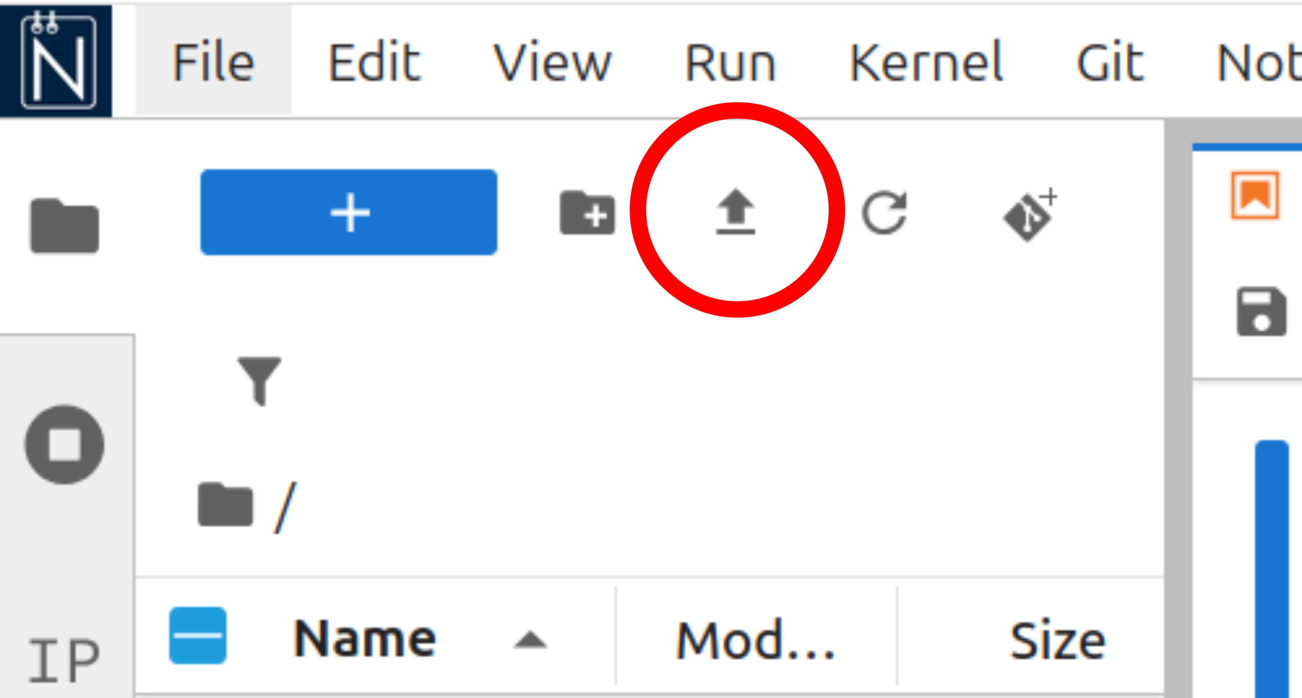
This session will require you to download files from this website and upload them to Noteable. To first download a file, left click on the hyperlink in the text - the file will be automatically downloaded to your computer. To then upload the file to noteable, use the upload button in the file browser window, as shown below, in red.
Reading a file
The most general way to read data from a file in Python is to use the built-in open function. Let’s look at a simple example: reading in a file that contains some simple text. We’re going to look at the file example.txt, which looks like this:
EXAMPLE TEXT FILE

Here is some text.
Here is some more text.

Here is even more text.[example.txt]
To download this file, click here, and then upload the file to Noteable.
We can read this file into Python and print its content as follows.
with open('example.txt', 'r') as stream:
    lines = stream.readlines()

for line in lines:
    print(line, end='')
Let’s break this down into sections. First we use the with keyword which tells Python we’re going to be using some sort of external resource - something that isn’t within the notebook. For this reason with is a very powerful and complicated keyword, but in this course we’re only going to use it to open files.
The with keyword is immediately followed by a call to the open function where we provide the file name example.txt, and the mode we’d like open the file in. The mode argument controls what we are able to do with the file and has several choices, the three most useful for this course are
r- Read-onlyw- Write-onlya- Append (i.e. write to the end of the file)
This line then ends with an as keyword. This is a very similar in style to how we’ve used as when we use an import keyword, for example
import scipy.constants as constWe’re essentially nicknaming the output of open('example.txt', 'r') and calling it stream, a variable which contains all information about the file, but not necessarily in a human-readable format.
To obtain the contents of the file, we finish this line with a colon : just like in a for loop, and then indent the code and use the readlines method of the variable stream to obtain all of the lines in the file as a list of strings and assign this to the variable lines.
The remaining code simply prints each element of the lines list so that we can read it.
for line in lines:
    print(line, end='')
We have used the end keyword argument here just to prevent the print function from adding needless whitespace to the output (by default each line passed to print will be followed by a newline).
You might wonder why we’re using as and not = (the assignment operator). When we use with and as in this combination, we tell python to only keep the file open within the indented with block.
In our example we read all of the file into memory, but it can be more memory efficient to read the file line by line within the with block when the file you’re reading is quite large.
Writing files
Now that we’ve read in our simple text file, let’s make some modifications to it and write it back out again.
We now have the contents of the text file available to us in the form of a list of strings.
print(lines)\n is a newline character which will actually become a newline when passed to the print function.
Let’s make some changes to lines, starting by removing the last two lines.
lines = lines[:-2]and now add a new final line
lines.append('This new text was added in Python!')
print(lines)
['EXAMPLE TEXT FILE\n',
'\n',
'Here is some text.\n',
'Here is some more text.\n',
'This new text was added in Python!']Now we can write this to a new file
with open('modified_example.txt', 'w') as stream:
    for line in lines:
        stream.write(line)
You should now see the file modified_example.txt has been created in the same directory as your Jupyter notebook - look at the file browser on the left of your Noteable window.
This code is much like that used to read the original file, since we use with open() as to open the file and store information about it in the variable stream. The difference is that we use w as our second argument of open, and the write method of stream rather than the readlines method. We use a for loop to write each individual line from the elements of the list lines.
Typing
Notice that in the above example that the file’s contents are read in as strings. When using with open... the lines of the file are always read as strings, so if you wanted to read in a set of numbers you’d have to convert each str to a float or int.
For example, the following file contains three numbers on each line
1 2 3
1 4 9
1 8 27[example_numbers.txt]
To download this file, click here, and then upload the file to Noteable.
This could be read in using
with open('example_numbers.txt', 'r') as stream:
    lines = stream.readlines()

print(lines)
['1 2 3\n', '1 4 9\n', '1 8 27']but notice that, as we have already said, the data is contained in a set of strings.
To obtain a list of numeric types (float or int), we’d have to take each line, split it into three values, and then convert each value into either float or int objects.
values = []

for line in lines:
    values.append(
        [
            float(str_value)
            for str_value in line.split()
        ]
    )

print(values)
[[1.0, 2.0, 3.0], [1.0, 4.0, 9.0], [1.0, 8.0, 27.0]]The split() method of str splits the string at a specified character - if no character is given then the string is split up by whitespace and a list of the split strings is returned. To see this a little clearer, try the following
test = 'this is a test'
print(test.split())
Take a moment to read this code. All we want is to have the data from the file stored as float instead of str, but we’ve had to go through quite a convoluted process to get there. Thankfully, when a file is nicely structured like this one (3 rows and 3 columns of data) it can be read using a much simpler method as is shown below.
Reading in scientific data with NumPy
What we have just been through is the most general case: how to read in any file, regardless of what type of data is contained within. For our purposes, we are primarily interested in scientific data such as numbers that have been collected during some series of experiments. There are many Python packages that can be used to read such data, here we’re going to rely on the very popular NumPy package (“numeric Python”, pronounced numb-pie).
NumPy has a large number of functions and objects used for numerical methods (e.g. linear algebra, fourier transforms), but for now we’re just going to use it to load in a file.
In the following example, we have experimental data which gives the temperature dependence of the equilibrium constant for a reaction.You can download the file by clicking here, and then upload it to your Noteable file system.
This data is formatted as simple text in a table of sorts, with values on each line being separated by whitespace. Simple tabular data can be read from files like this using the loadtxt function
import numpy as np

data = np.loadtxt('thermodynamic_data.dat')

print(data)
type(data)
[[1.00e+02 2.38e+38]
[1.20e+02 2.15e+30]
[1.40e+02 3.86e+24]
[1.60e+02 1.89e+20]
[1.80e+02 8.42e+16]
[2.00e+02 1.75e+14]
[2.20e+02 1.12e+12]
[2.40e+02 1.67e+10]
[2.60e+02 4.73e+08]
[2.80e+02 2.24e+07]
[3.00e+02 1.59e+06]
[3.20e+02 1.57e+05]
[3.40e+02 2.03e+04]
[3.60e+02 3.30e+03]
[3.80e+02 6.50e+02]
[4.00e+02 1.51e+02]
[4.20e+02 4.01e+01]
[4.40e+02 1.21e+01]
[4.60e+02 4.02e+00]
[4.80e+02 1.47e+00]
[5.00e+02 5.82e-01]]
numpy.ndarrayWhen we use import numpy as np what we’re saying is that we’d like to use NumPy but rename it to np. This is a choice - we could give it any name we like!
However Python programmers nearly always import numpy as np - for some reason this is a convention that has stuck! While completely allowed, it’s incredibly rare to see it imported as any other name.
The data is read from the file and stored in a variable called data - notice this is much simpler than using with open...!
The variable data is a new type: a NumPy ndarray (often just called a NumPy array). You can think of NumPy arrays as being a bit like a list, but with added features - we’ll see some of these later on in this session. One important thing to realise is that NumPy arrays are not a built-in type in Python, they’re a feature of the NumPy package that we’ve imported.
One thing we can see is that this array is two dimensional, since we have a lots of entries like [1.00e+02 2.38e+38] all enclosed in an outer set of square brackets. We can describe this data as having rows and columns, much like a table or matrix.
As written above, each pair of values is a single temperature and a single equilibrium constant. We therefore have 21 columns with two rows - this is a little bit hard to think about, but if we think of this as a table (which is basically is) the data is currently written like this
| Column 1 | Column 2 | Column 3 | Column 4 | Column 5 | Column 6 | Column 7 | Column 8 | Column 9 | Column 10 | Column 11 | Column 12 | Column 13 | Column 14 | Column 15 | Column 16 | Column 17 | Column 18 | Column 19 | Column 20 | Column 21 | |
|---|---|---|---|---|---|---|---|---|---|---|---|---|---|---|---|---|---|---|---|---|---|
| \(T\mathrm{ / K}\) | 1.00e+02 | 1.20e+02 | 1.40e+02 | 1.60e+02 | 1.80e+02 | 2.00e+02 | 2.20e+02 | 2.40e+02 | 2.60e+02 | 2.80e+02 | 3.00e+02 | 3.20e+02 | 3.40e+02 | 3.60e+02 | 3.80e+02 | 4.00e+02 | 4.20e+02 | 4.40e+02 | 4.60e+02 | 4.80e+02 | 5.00e+02 |
| \(K\) | 2.38e+38 | 2.15e+30 | 3.86e+24 | 1.89e+20 | 8.42e+16 | 1.75e+14 | 1.12e+12 | 1.67e+10 | 4.73e+08 | 2.24e+07 | 1.59e+06 | 1.57e+05 | 2.03e+04 | 3.30e+03 | 6.50e+02 | 1.51e+02 | 4.01e+01 | 1.21e+01 | 4.02e+00 | 1.47e+00 | 5.82e-01 |
As you can see this is a very strange (and annoying!) layout. To fix this we can transpose the data, swapping rows for columns and vice-versa. To do this, we use the T method of the NumPy array
transposed_data = data.T

print(transposed_data)
[[1.00e+02 1.20e+02 1.40e+02 1.60e+02 1.80e+02 2.00e+02 2.20e+02 2.40e+02
2.60e+02 2.80e+02 3.00e+02 3.20e+02 3.40e+02 3.60e+02 3.80e+02 4.00e+02
4.20e+02 4.40e+02 4.60e+02 4.80e+02 5.00e+02]
[2.38e+38 2.15e+30 3.86e+24 1.89e+20 8.42e+16 1.75e+14 1.12e+12 1.67e+10
4.73e+08 2.24e+07 1.59e+06 1.57e+05 2.03e+04 3.30e+03 6.50e+02 1.51e+02
4.01e+01 1.21e+01 4.02e+00 1.47e+00 5.82e-01]]Where we now have two columns, each with 21 entries each. The first column is the temperature, and the second column is the equilibrium constant. This could be written in a table as
| \(T\mathrm{ / K}\) | \(K\) |
|---|---|
| 1.00e+02 | 2.38e+38 |
| 1.20e+02 | 2.15e+30 |
| 1.40e+02 | 3.86e+24 |
| 1.60e+02 | 1.89e+20 |
| 1.80e+02 | 8.42e+16 |
| 2.00e+02 | 1.75e+14 |
| 2.20e+02 | 1.12e+12 |
| 2.40e+02 | 1.67e+10 |
| 2.60e+02 | 4.73e+08 |
| 2.80e+02 | 2.24e+07 |
| 3.00e+02 | 1.59e+06 |
| 3.20e+02 | 1.57e+05 |
| 3.40e+02 | 2.03e+04 |
| 3.60e+02 | 3.30e+03 |
| 3.80e+02 | 6.50e+02 |
| 4.00e+02 | 1.51e+02 |
| 4.20e+02 | 4.01e+01 |
| 4.40e+02 | 1.21e+01 |
| 4.60e+02 | 4.02e+00 |
| 4.80e+02 | 1.47e+00 |
| 5.00e+02 | 5.82e-01 |
Which is much more sensible!
We can avoid all of this entirely if we use the unpack keyword when calling np.loadtxt.
temperature, K = np.loadtxt('thermodynamic_data.dat', unpack=True)

print(temperature)
print(K)
This keyword argument tells Python to take each column of data from the file and place them into separate NumPy arrays which are then stored in the arrays temperature and K respectively.
Remember that Python doesn’t “know” what your file contains. If you want the temperature array to contain temperatures then the temperature data must be the first column of your file. Similarly the equilibrium constants must be the second column.
For one final example, let’s look at reading in a csv (comma-separated-variable) file.
csv files contain data separated (or delimited) by commas rather than whitespace.
Click here to download a csv file.
To read in this csv file, we need to tell NumPy that the file is separated by commas, otherwise loadtxt will fail.
temperature, K = np.loadtxt('thermodynamic_data.csv', unpack=True, delimiter=',')

print(temperature)
print(K)
By setting the delimiter to a comma ,, the loadtxt function is able to successfully parse the data and we end up with the same result as our previous example using thermodynamic_data.dat.
Writing data with NumPy
NumPy also provides us with a simple function for writing data to a file - np.savetxt.
Say we want to use the data in thermodynamic_data.csv and calculate the change in Gibbs’ free energy associated with each pair of equilibrium constant and temperature values. We could do this relatively easily
from scipy import constants

# Load in the file containing temperature and equilibrium constants and create
# an array for each quantity.
temperature, K = np.loadtxt('thermodynamic_data.csv', unpack=True, delimiter=',')

# Calculate change in Gibbs' free energy and store in an array
# Delta G = -R T ln(K)
DG = -constants.R * temperature * np.log(K)
# Convert to kJ mol-1
DG *= 1E-3
print(DG)
To save this to a file we can use the following piece of code
np.savetxt(
    'full_thermodynamic_data.csv',
    np.array([temperature, K, DG]).T,
    delimiter=',',
    header='Temperature (K), Equilibrium Constant, Delta G (kJ mol-1)'
)
Let’s break this down, argument by argument
The first argument contains the name of the output file. We’ve specified a
.csvextension, so later on we’ll have to tellnp.savetxtto use a comma as the delimiter.The second argument contains the array we want to save. Here we want the temperatures, equilibrium constants, and changes in Gibbs’ free energy as individual columns in our file. To achieve this, we create a NumPy array whose elements are the
temperature,KandDGarrays, and then take its transpose using the.Tmethod. If we didn’t take the transpose we’d end up with a file containing three rows of data as opposed to three columns.The third argument uses the
delimiterkeyword to specify which character to use as a delimiter - here this is a comma,since we’ve used the.csvfile extension.The final argument uses the
headerkeyword to write some text to our file - this is a very important step, since it allows anyone who opens the file to know what each column contains. When the file is written, this row will begin with a#character, symbolising that it is a comment row or header.
When this code is executed, the file full_thermodynamic_data.csv is created and saved to Noteable’s filesystem. You can open the file by double clicking on its name in the file browser, and should see the following:
# Temperature (K), Equilibrium Constant, Delta G (kJ mol-1)
1.000000000000000000e+02,2.380000000000000086e+38,-7.347102664620298640e+01
1.200000000000000000e+02,2.150000000000000001e+30,-6.968486210200136100e+01
1.400000000000000000e+02,3.859999999999999925e+24,-6.589859586046311790e+01
1.600000000000000000e+02,1.890000000000000000e+20,-6.211007165843453492e+01
1.800000000000000000e+02,8.420000000000000000e+16,-5.832557975950992102e+01
2.000000000000000000e+02,1.750000000000000000e+14,-5.453590241614799083e+01
2.200000000000000000e+02,1.120000000000000000e+12,-5.074945904321485557e+01
2.400000000000000000e+02,1.670000000000000000e+10,-4.697074312315339739e+01
2.600000000000000000e+02,4.730000000000000000e+08,-4.318030975807940308e+01
2.800000000000000000e+02,2.240000000000000000e+07,-3.940124081737333483e+01
3.000000000000000000e+02,1.590000000000000000e+06,-3.561727356828706803e+01
3.200000000000000000e+02,1.570000000000000000e+05,-3.183175672934730116e+01
3.400000000000000000e+02,2.030000000000000000e+04,-2.803842907135382134e+01
3.600000000000000000e+02,3.300000000000000000e+03,-2.424999483919259191e+01
3.800000000000000000e+02,6.500000000000000000e+02,-2.046396694422201179e+01
4.000000000000000000e+02,1.510000000000000000e+02,-1.668639425920466834e+01
4.200000000000000000e+02,4.010000000000000142e+01,-1.289056042729434637e+01
4.400000000000000000e+02,1.209999999999999964e+01,-9.121051955418014501e+00
4.600000000000000000e+02,4.019999999999999574e+00,-5.321170230539470580e+00
4.800000000000000000e+02,1.469999999999999973e+00,-1.537559918185818386e+00
5.000000000000000000e+02,5.819999999999999618e-01,2.250246247603662209e+00