Mini Project
Before your proper group projects begin, we’ll spend this session using all of the Python skills you’ve developed so far to solve a real chemical problem.
We’ll step through the problem slowly, and you’ll be provided with hints for each part.
You MUST fill out the group project choice form (once per group) by 12:00pm (midday) on Friday 13th March.
You can find the form on the CH12004 Moodle page.
The problem
Blue-1 is a water-soluble dye which has been used in food, drugs, and cosmetics due to its vibrant blue colour. The UV-Visible spectrum of Blue-1 contains an intense peak at \(627\, \mathrm{nm}\).
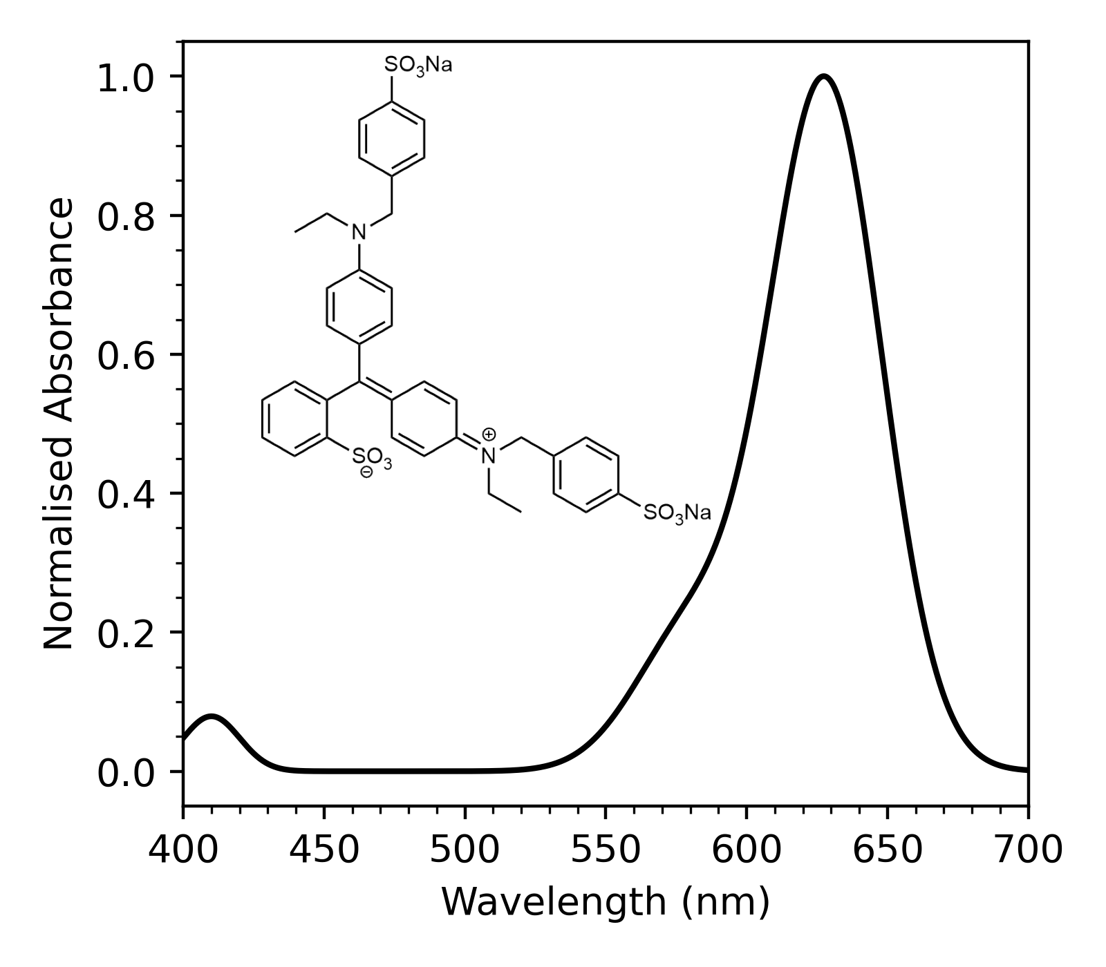
The absorption corresponds to the excitation of an electron from a filled orbital of the \(\pi\) system to an empty orbital, and is sensitive to the energy and composition of the \(\pi\) orbitals of Blue-1.
Blue-1 reacts with bleach (a strong oxidising agent) to produce a complex mixture of completely colourless products
\[\begin{equation*} \mathrm{dye}\ +\ \mathrm{bleach}\ \rightarrow\ \mathrm{colorless\ products} \end{equation*}\]
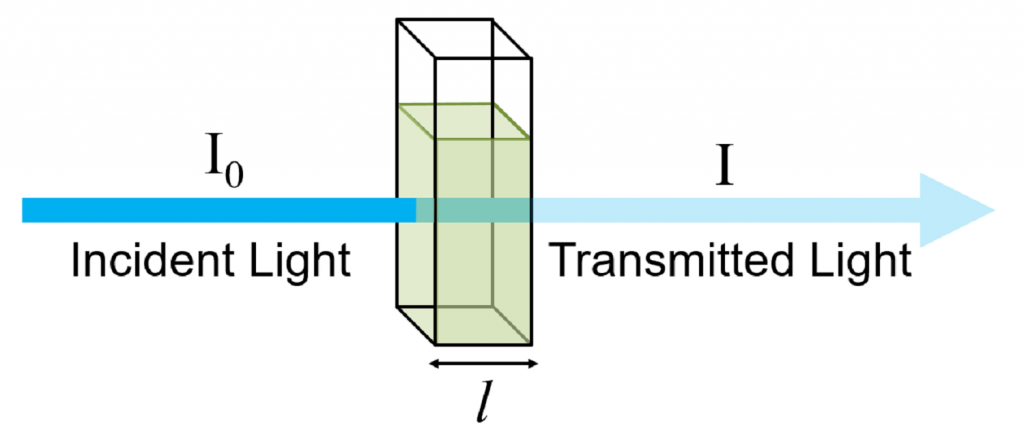
For a given sample, its absorbance \(A\) (at a given wavelength) is the ratio of incident \(I_0\) to transmitted \(I\) light intensity.
\[\begin{equation*} A = \log_{10}\left(\frac{I_0}{I}\right) \end{equation*}\]
The Beer-Lambert law states that the absorbance of a solution-phase sample is also directly proportional to the concentration \(c\) of the solution, the path length \(l\), and a sample- and wavelength-dependent proportionality constant \(\varepsilon\) called the molar extinction coefficient.
\[\begin{equation*} A = \varepsilon c l \end{equation*}\]
If we wish to study the kinetics of the solution-phase reaction of bleach and Blue-1 then we can exploit this relationship between absorbance and concentration by recording the UV-Visible spectrum over the course of the reaction.
We can write the rate of reaction as
\[\begin{equation*} \nu = k[\mathrm{dye}]^n[\mathrm{bleach}]^m \end{equation*}\]
where \(n\) and \(m\) are unknown orders of reaction for either reactant.
The concentration of bleach is much larger than that of the dye, so we can write
\[\begin{equation*} k' = k[\mathrm{bleach}]^m \qquad \nu = k'[\mathrm{dye}]^n \end{equation*}\]
where \(k'\) is a pseudo rate constant.
In this mini-project you will use multiple UV-visible spectra of Blue-1, each recorded at a specific point of time during the reaction, to obtain
- The order of reaction \(n\) with respect to Blue-1
- The pseudo rate constant \(k'\)
The three values of \(n\) you should consider are summarised in the Table below. These correspond to zeroth-, first-, and second-order reactions with respect to the concentration of Blue-1.
| \(n\) | Rate Law | (Linear) Integrated Rate Law | |
|---|---|---|---|
| 0 | \(v = k'\) | \([\mathrm{dye}]_t = -k't + [\mathrm{dye}]_0\) | |
| 1 | \(\nu = k'[\mathrm{dye}]\) | \(\ln([\mathrm{dye}]_t) = -k't + \ln([\mathrm{dye}]_0)\) | |
| 2 | \(\nu = k'[\mathrm{dye}]^2\) | \(\frac{1}{[\mathrm{dye}]_t} = k't + \frac{1}{[\mathrm{dye}]_0}\) |
You have been provided with 41 .csv files, each containing a single spectrum recorded at a specific point of time during the reaction, where the time value is stored in the file name. For example, t_0p5.csv corresponds to \(t = 0.5 \mathrm{\ s}\), i.e. the p means decimal point. The spectra you have been given have been recorded from \(t=0 \mathrm{\ s}\) to \(t=20 \mathrm{\ s}\) in steps of \(0.5\mathrm{\ s}\).
Use this as an opportunity to prepare for your group projects by writing a notebook that not only contains code, but also explains your methodology and results.
Make sure to use all of the programming skills you’ve developed, write readable code, and employ Markdown cells and formatting where appropriate.
Step 0: Uploading files
Since there are a lot of files, you’re going to upload this zip to Noteable, and then run this command in a new cell, on its own, to unzip file files.
!unzip uv_vis_data.zip -d .You should then see the directory uv_vis_data inside of the file browser - this is where the data will be read from.
Finally, delete the cell that contains the above code - you shouldn’t need it again.
Step 1: Plotting the initial spectrum
Let’s start with something simple - plotting the spectrum at \(t=0\).
First, load the data from the file t_0p0.csv. Since this file is inside of a directory (also known as a folder), you’ll need to include the folder name as follows when using np.loadtxt.
'uv_vis_data/t_0p0.csv'Now plot this spectrum as normalised absorbance as a function of wavelength - make sure to follow the advice in plotting tips.
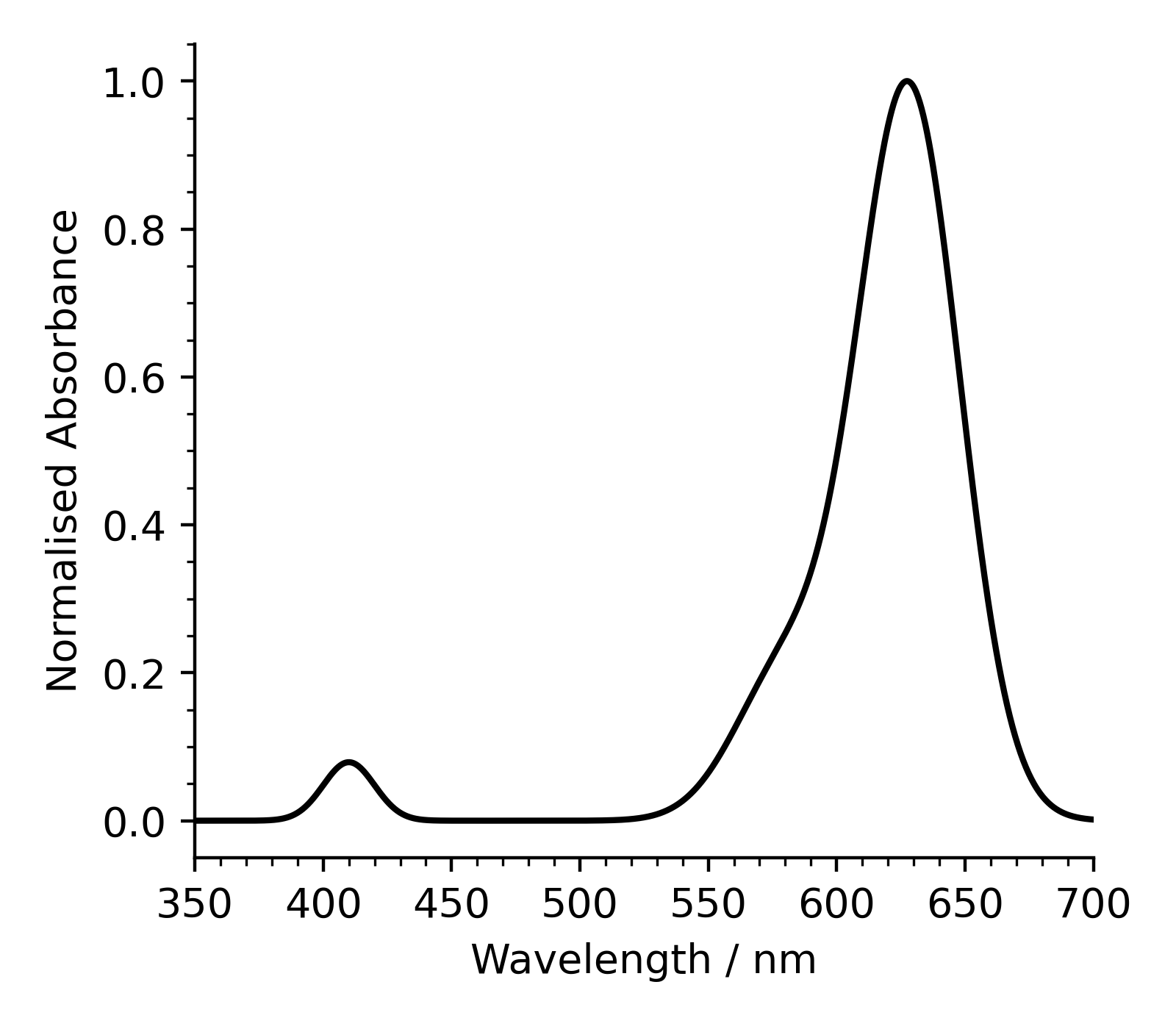
Your figure should look similar to the one below.
Normalised absorbance means that the data has been scaled such that the “height” of the tallest peak is set to 1.
In this dataset, all spectra have been scaled relative to the height of the tallest peak in the spectrum for \(t=0\).
We have a strong signal at \(627 \mathrm{\ nm}\), this is the one we’ll track over the course of the reaction.
Step 2: Plotting all spectra
Using your code from Step 1 as a starting point, plot all of the spectra in a single figure. To highlight the difference between the spectra, you can modify the transparency of each line.
The following piece of code generates a list of 41 colors with decreasing opacity, each of which can be passed to the color keyword argument of ax.plot.
# Make list of black colours, changing only the alpha, aka transparency
# of the colour
colours = [
    ("#000000", alpha)
    for alpha in np.logspace(0, -1.8, 41)
]
Your figure should look similar to the one below.
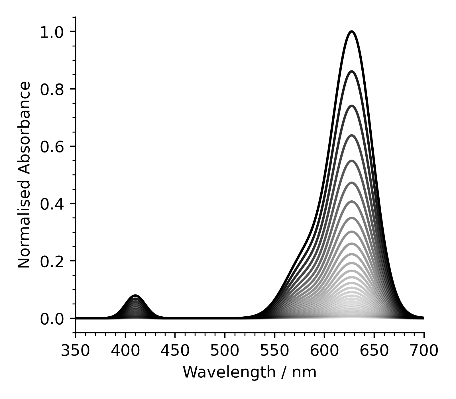
You’ll need to modify your code to loop over every file name - think about how you could write code to construct a list of the file names.
The intensity drops over time, as more and more of the Blue-1 present in the solution is oxidised by the bleach.
Step 3: Converting intensity to concentration
Now that we know what the spectra look like, we can start to process them and understand how the concentration changes as a function of time.
We can use the Beer-Lambert law to relate the concentration of Blue-1 present to the absorbance at \(\sim 627 \mathrm{\ nm}\). If we have an initial Blue-1 concentration of \([\mathrm{dye}]_0 = c_0\), then the initial absorbance will be
\[\begin{equation*} A_0 = \varepsilon c_0 l = \varepsilon [\mathrm{dye}]_0 l \end{equation*}\]
If we divide the absorbance of each spectrum taken at a time \(t\) by \(A_0\), then
\[\begin{equation*} \frac{A_t}{A_0} = \frac{\varepsilon [\mathrm{dye}]_t l}{\varepsilon [\mathrm{dye}]_0 l} = \frac{[\mathrm{dye}]_t}{[\mathrm{dye}]_0} \end{equation*}\]
where the measured solution had an initial Blue-1 (dye) concentration of \(10\ \mathrm{\mu M}\).
Using the above information and the spectral data files, calculate the concentration of dye present at the time of each measurement, and plot the dye concentration as a function of time in a figure.
You’ll need to obtain the absorbance at the peak maximum (\(\sim 627 \mathrm{\ nm}\)) for each measurement. This can be done in a variety of ways, but it may help you to know that, thankfully, the strongest peak in your spectrum is always the one at roughly \(627 \mathrm{\ nm}\).
Your figure should look similar to the one below.
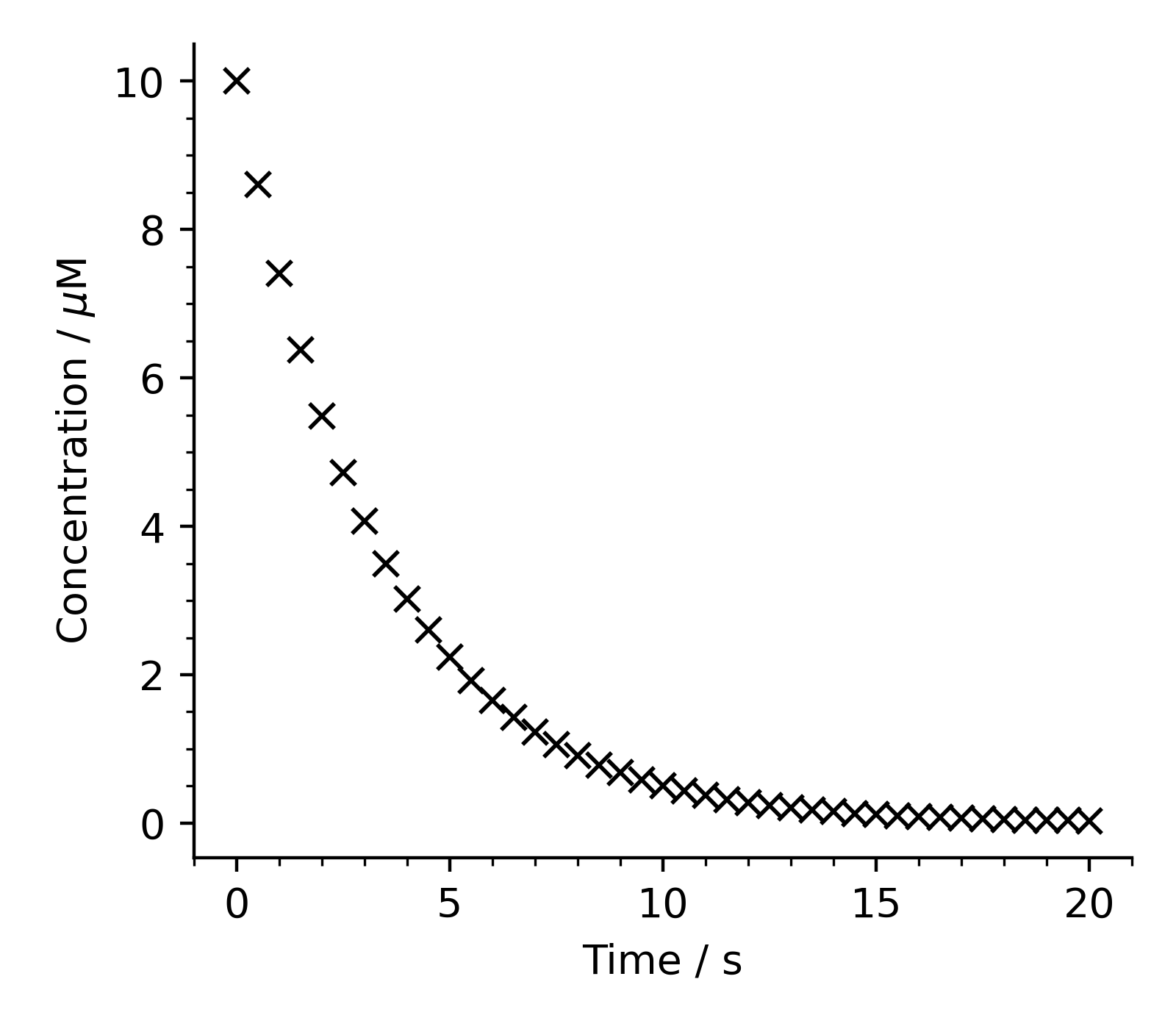
So the concentration decreases over time as more Blue-1 reacts with bleach - hardly a surprising observation!
Step 4: Obtaining the order of reaction
We now need to decide the order of reaction with respect to the concentration of dye. If we assume that this is an elementary reaction then we may limit ourselves to integer orders (Table 1).
Take the second-order integrated rate equation as an example
\[\begin{equation*} \color{red}{\frac{1}{[\mathrm{dye}]_t}} = \color{blue}{k'}\color{ForestGreen}{t} + \color{purple}{\frac{1}{[\mathrm{dye}]_0}} \end{equation*}\]
This has the same form as the equation of a straight line
\[\begin{equation*} \color{red}{y} = \color{blue}{m}\color{ForestGreen}{x} + \color{purple}{c} \end{equation*}\]
A plot of \(\color{red}{\frac{1}{[\mathrm{dye}]_t}}\) against \(\color{ForestGreen}{t}\) will therefore be linear if the reaction has second-order kinetics with respect to dye concentration.
Carry out this process for zeroth-, first-, and second-order with respect to dye concentration. Based on your results, which order do you think is the most appropriate?
Step 5: Determining the pseudo rate constant
Now that you know the order of reaction with respect to dye concentration, you should fit your chosen model to the data. From this fit you can obtain the pseudo rate constant \(k'\), its standard deviation, and a goodness of fit statistic which describes the quality of your fit.
To do this, use Ordinary Least Squares (OLS) regression, as covered in Session 6.
Comment on your fitted values, how could you improve their accuracy?
Example notebook
You can download an example notebook which attempts this mini-project here (you’ll need to upload the file to noteable to view it properly). You should use this as a starting point for how to construct your group notebook in your project.