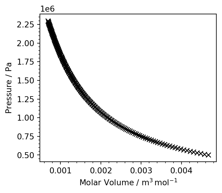
a. Read in the experimental data using NumPy, convert each quantity to SI units, and plot the isotherm using Matplotlib.
import matplotlib.pyplot as pltimport numpy as np%config InlineBackend.figure_format='retina'# Load dataexp_p, exp_vm = np.loadtxt('isotherm.csv', unpack=True, delimiter=',')# Convert from bar to Paexp_p *=1E5# Convert from L mol^-1 to m^3 mol^-1exp_vm *=1E-3fig, ax = plt.subplots(nrows=1, ncols=1, figsize=(4, 3.5))ax.plot(exp_vm, exp_p, lw=0, marker='x', color='k')ax.set_xlabel(r'Molar Volume / $\mathregular{m^3\, mol^{-1}}$')ax.set_ylabel(r'Pressure / $\mathregular{Pa}$')ax.minorticks_on()fig.tight_layout()plt.show()
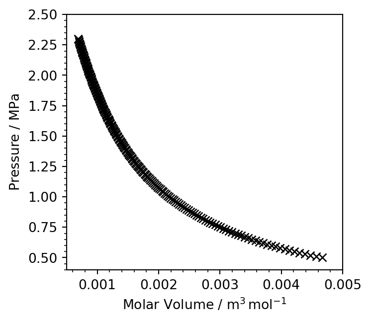
To make this plot even better, we can adjust the axis limits to include some more numbered ticks. We can also change the pressure values so that they’re in units of \(\mathrm{MPa}\) - this avoids the odd 1e6 at the top of the figure.
fig, ax = plt.subplots(nrows=1, ncols=1, figsize=(4, 3.5))ax.plot(exp_vm, exp_p *1E-6, lw=0, marker='x', color='k')ax.set_xlabel(r'Molar Volume / $\mathregular{m^3\, mol^{-1}}$')ax.set_ylabel(r'Pressure / $\mathregular{MPa}$')ax.minorticks_on()# Set limits to more sensible valuesax.set_xlim(0.0005, 0.005)ax.set_ylim(0.4, 2.5)fig.tight_layout()plt.show()
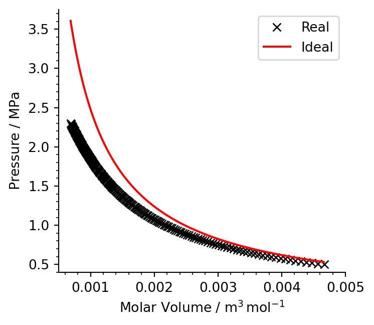
b. Assuming ideality, the isotherm should be well modelled by the ideal gas law:
\[p = \frac{RT}{V_\mathrm{m}},\]
where \(p\) is the pressure, \(V_\mathrm{m}\) is the molar volume (\(V / n\)), \(R\) is the gas constant and \(T\) is the temperature.
Write a function to calculate the pressure with the ideal gas law and use this to model the \(\ce{SF6}\) isotherm between \(V_\mathrm{m} = 6.87 \times 10^{-4}\,\mathrm{m}^{3}\,\mathrm{mol}^{-1}\) and \(V_\mathrm{m} = 4.66 \times 10^{-3}\,\mathrm{m}^{3}\,\mathrm{mol}^{-1}\). Plot your modelled isotherm against the experimental data.
import scipy.constants as constantsdef calc_ideal_gas_pressure(Vm, T):''' Calculates the ideal gas pressure for a given molar volume and temperature Arguments --------- Vm: float | np.ndarray Molar volume in m^3 mol^-1 T: float Temperature in Kelvin Returns ------- float | np.ndarray Ideal gas pressure '''return constants.R * T / Vm# Ideal molar volumeideal_vm = np.linspace(6.87E-4, 4.66E-3, 1000)# Temperature in Kelvintemperature =298# Calculate ideal gas pressureideal_p = calc_ideal_gas_pressure(ideal_vm, temperature)# Create plotfig, ax = plt.subplots(nrows=1, ncols=1, figsize=(4, 3.5))# plot experimentax.plot(exp_vm, exp_p *1E-6, lw=0, marker='x', color='k', label='Real')# plot ideal gas valuesax.plot(ideal_vm, ideal_p *1E-6, color='r', label='Ideal')ax.set_xlabel(r'Molar Volume / $\mathregular{m^3\, mol^{-1}}$')ax.set_ylabel(r'Pressure / $\mathregular{MPa}$')ax.minorticks_on()ax.legend()# Set limits to more sensible valuesax.set_xlim(0.0005, 0.005)ax.set_ylim(0.4, 3.75)ax.spines[['top', 'right']].set_visible(False)fig.tight_layout()plt.show()
Notice that we have again adjusted the y axis, this time so that we can see the all points along the ideal isotherm.
c. Non-ideality due to intermolecular interactions and other factors can be accounted for (in part) by the Van der Waals equation of state:
where \(p\) is the pressure, \(R\) is the gas constant, \(V_\mathrm{m}\) is the molar volume and \(a\) and \(b\) are system dependent constants that describe the strength of the interactions and excluded volume effects respectively.
Write a function to calculate the pressure with the Van der Waals equation and use this to model the \(\ce{SF6}\) isotherm using
\[\begin{equation*}
a = 7.857 \times 10^{-1}\,\mathrm{m}^6\,\mathrm{Pa\, mol}^{-2} \qquad b = 8.79 \times 10^{-5}\,\mathrm{m}^3\,\mathrm{mol}^{-1}
\end{equation*}\]
between \(V_\mathrm{m} = 6.87 \times 10^{-4}\,\mathrm{m}^3\,\mathrm{mol}^{-1}\) and \(V_\mathrm{m} = 4.66 \times 10^{-3}\,\mathrm{m}^3\,\mathrm{mol}^{-1}\).
Plot your modelled isotherm and compare this against the idealised curve and the experimental data.
def calc_vdw_gas_pressure(Vm, T, a, b):''' Calculates the gas pressure for a given molar volume and temperature using the Van der Waals equation of state\n p = RT/(Vm - b) - a/(Vm^2) Arguments --------- Vm: float | np.ndarray Molar volume in m^3 mol^-1 T: float Temperature in Kelvin a: float Van der Waals a constant b: float Van der Waals b constant Returns ------- float | np.ndarray Gas pressure according to Van der Waals equation '''return constants.R * T / (Vm - b) - a / Vm**2# Van der Waals molar volumevdw_vm = np.linspace(6.87E-4, 4.66E-3, 1000)# Temperature in Kelvintemperature =298# Van der Waals equation constants for SF6a =0.7857# m^6 Pa mol^-2b =8.79E-5# m^3 mol^-1# Calculate ideal gas pressurevdw_p = calc_vdw_gas_pressure(ideal_vm, temperature, a, b)# Create plotfig, ax = plt.subplots(nrows=1, ncols=1, figsize=(4, 3.5))# plot experimentax.plot(exp_vm, exp_p *1E-6, lw=0, marker='x', color='k', label='Real')# plot ideal gas valuesax.plot(ideal_vm, ideal_p *1E-6, color='r', label='Ideal')# plot ideal gas valuesax.plot(vdw_vm, vdw_p *1E-6, color='C0', label='Van der Waals')ax.set_xlabel(r'Molar Volume / $\mathregular{m^3\, mol^{-1}}$')ax.set_ylabel(r'Pressure / $\mathregular{MPa}$')ax.minorticks_on()ax.legend()# Set limits to more sensible valuesax.set_xlim(0.0005, 0.005)ax.set_ylim(0.4, 3.75)ax.spines[['top', 'right']].set_visible(False)fig.tight_layout()plt.show()
So the Van der Waals equation is an improvement over the ideal gas model, just as you’ve been taught.
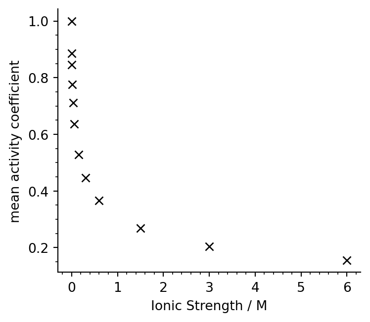
2. The mean activity coefficient of ions in solution can be measured experimentally. You have been provided with the mean activity coefficient of \(\ce{Na2SO4}\) at \(298\,\mathrm{K}\) for a range of ionic strengths.
a. Use Matplotlib to create a scatter plot of the experimental mean activity coefficient as a function of the ionic strength \(I\).
b. The mean activity coefficient can be predicted by the Debye-Huckel limiting law:
\[\ln\gamma_{\pm} = -|z_{+}z_{-}|A\sqrt{I},\]
where \(z_{+}\) and \(z_{-}\) are cation and anion charges, \(I\) is the ionic strength and \(A\) is a solvent- and temperature-dependent constant.
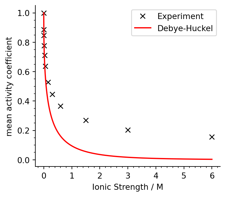
Write a function to calculate the mean activity coefficient according to the Debye-Huckel limiting law (feel free to reuse your code from previous exercises). Using \(A = 1.179\,\mathrm{M}^{-\frac{1}{2}}\), plot the Debye-Huckel mean activity coefficient between \(I = 0\,\mathrm{M}\) and \(I = 6\,\mathrm{M}\) and compare this with the experimental values.
def calc_debye_huckel_gamma(I, z_plus, z_minus, A):''' Calculates mean activity coefficient according to Debye-Huckel equation Arguments --------- I: float Molar Ionic Strength in M z_plus: int Charge of positive ion z_minus: int Charge of negative ion A: float Debye-Huckel constant in M^{-1/2} Returns ------- float | np.ndarray Mean activity coefficient '''return np.exp(-abs(z_plus * z_minus) * A * np.sqrt(I))dh_I = np.linspace(0, 6, 1000)dh_gamma = calc_debye_huckel_gamma(dh_I, 1, -2, 1.179)# Create plotfig, ax = plt.subplots(nrows=1, ncols=1, figsize=(4, 3.5))# Plot experimental dataax.plot(exp_I, exp_gamma, lw=0, marker='x', color='k', label='Experiment')# Plot Debye-Huckel valuesax.plot(dh_I, dh_gamma, color='r', label='Debye-Huckel')ax.set_xlabel(r'Ionic Strength / M')ax.set_ylabel(r'mean activity coefficient')ax.minorticks_on()ax.legend()ax.spines[['top', 'right']].set_visible(False)fig.tight_layout()plt.show()
Notice that the Debye-Huckel limiting law is very inaccurate when the solution is not dilute (i.e. it does not behave as an Ideal-Dilute solution).
c. There are several extensions of the Debye-Huckel limiting law that aim to improve its description of the mean activity coefficient outside of the dilute limit. One such extension is:
where \(B\) is another solvent- and temperature-dependent constant and \(a_{0}\) is the distance of closest approach (expected to be proportional to the closest distance between ions in solution).
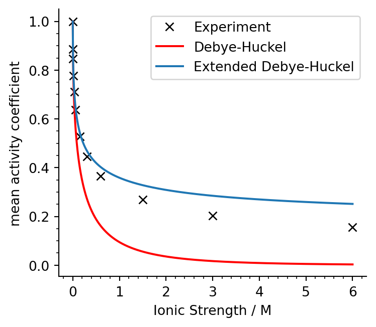
Write a function to calculate the mean activity coefficient according to the extended Debye-Huckel limiting law. Using
plot the extended Debye-Huckel mean activity coefficient between \(I = 0\,\mathrm{M}\) and \(I = 6\,\mathrm{M}\) and compare this with the experimental values and the original Debye-Huckel limiting law.
def calc_extended_debye_huckel_gamma(I, z_plus, z_minus, A, B, a0):''' Calculates mean activity coefficient according to extended Debye-Huckel equation Arguments --------- I: float Molar Ionic Strength in M z_plus: int Charge of positive ion z_minus: int Charge of negative ion A: float Debye-Huckel constant in M^{-1/2} B: float Extended Debye-Huckel constant B in nm^-1 M^-1/2 a0: float Extended Debye-Huckel constant a0 in nm Returns ------- float | np.ndarray Mean activity coefficient ''' gamma_pm =-abs(z_plus * z_minus) gamma_pm *= ((A * np.sqrt(I)) / (1+ B * a0 * np.sqrt(I))) gamma_pm = np.exp(gamma_pm)return gamma_pmedh_I = np.linspace(0, 6, 1000)edh_gamma = calc_extended_debye_huckel_gamma(edh_I, 1, -2, 1.179, 18.3, 0.071)# Create plotfig, ax = plt.subplots(nrows=1, ncols=1, figsize=(4, 3.5))# Plot experimental dataax.plot(exp_I, exp_gamma, lw=0, marker='x', color='k', label='Experiment')# Plot Debye-Huckel valuesax.plot(dh_I, dh_gamma, color='r', label='Debye-Huckel')# Plot Extended Debye-Huckel valuesax.plot(edh_I, edh_gamma, color='C0', label='Extended Debye-Huckel')ax.set_xlabel(r'Ionic Strength / M')ax.set_ylabel(r'mean activity coefficient')ax.minorticks_on()ax.legend()ax.spines[['top', 'right']].set_visible(False)fig.tight_layout()plt.show()
The extended Debye-Huckel equation is a more accurate model when applied to more concentrated electrolyte solutions.