While it is very tempting to use the default plotting settings in Matplotlib, often a little bit of customisation can really improve the quality of a figure.
Choosing an appropriate size of figure
The size you choose in plt.subplots(figsize=(width, height)) is important - simply stretching or scaling your figure after the fact leads to low resolution images, or incorrectly sized text.
Up until now, we’ve used figsize=(4, 3.5) to make a figure with a width of 4 inches and a height of 3.5 inches. This is a good general purpose size, but won’t always be a good choice. Think about an NMR spectrum - this is usually shown in a wide and short figure.
Think wisely about the shape of your figure - what shape is typically used for the data you’re working with?
You should also consider how large your figure will be when placed into a word processor or presentation - see the section at the bottom of this page for more on this.
Choosing appropriate axis labels
Axis labels need to actually describe the quantity that is being plotted, otherwise they’re meaningless. They should always include units (when appropriate), and those units should be correctly formatted to use super- and sub-scripts, Greek symbols, etc.
Matplotlib allows us to use Mathtext to format mathematical symbols and operators.
Important
Be careful when formatting axis labels, variables, and units. The following rules always apply:
Variables should always be italic – \(x\) not x.
Units should always be Roman (non-italic), never italic, e.g. \(\mathrm{mol\, dm^{-3}}\) and not \(mol\, dm^{-3}\). Remember that you can obtain Roman characters in Mathtext using $\mathrm{}$.
Units should be separated by a small space - this can be specified in Mathtext using '$\,$' as, by default, spaces are ignored in Mathtext. e.g $\mathrm{mol\, dm^{-3}}$ and not $\mathrm{mol dm^{-3}}$
Subscripts should be italic when referring to a variable, and Roman when referring to anything else. For example, Avogadro’s constant is \(N_\mathrm{A}\) where the \(N\) is italic because it refers to the concept of a “number”, and the subscript \(\mathrm{A}\) is Roman because it literally means the name Avogadro.
Titles - do you really need one?
In School, you may have been told that “graphs” (or plots/figures) always need a title, usually beginning with “A graph to show.” Unfortunately, this is completely incorrect.
A brief look at pretty much any scientific paper demonstrates that titles are quite rarely included. The proper ways to include information on “what” you’re plotting are:
Correct axis labels.
Correct legend entries.
A good caption below your figure.
There’s no need to have a title which needlessly restates these things.
Titles might be useful when many subplots are present in a figure, and can be included with ax.set_title.
Choosing appropriate colours
The default Matplotlib colours are quite good for a quick plot, and in fact are colourblind friendly!
When plotting a single set of data, we recommend you use black markers or a black line - the colour is not required.
Save colours for emphasis, such as when plotting sets of data which vary due to an external factor - e.g. data for different molecules. These colours should be clearly distinguishable - i.e. not blue and purple.
Also consider whether your chosen colour is visible on a white background - bright green and bright yellow are rarely good choices!
It’s also nice to set your axis limits so that the data always appears within the tick marks, and never outside of it.
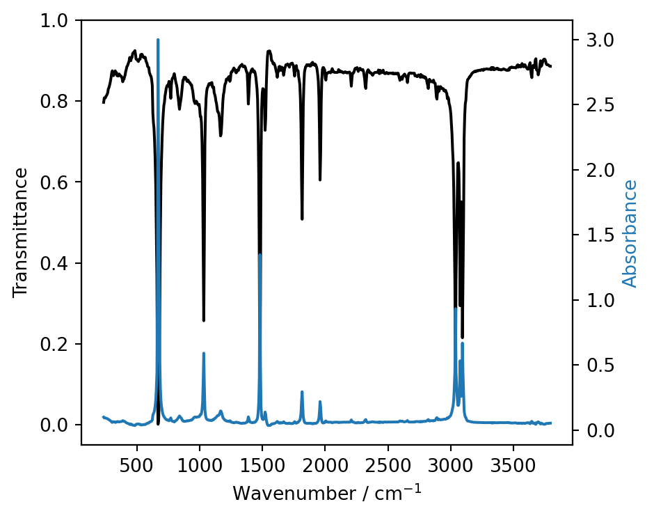
import matplotlib.pyplot as pltimport numpy as np%config InlineBackend.figure_format='retina'# Load the infrared data from filewavenumber, transmittance, absorbance = np.loadtxt('water_ir_spectrum.dat', unpack=True, skiprows=1)# Create the figure and the axesfig, ax = plt.subplots(figsize=(5, 4))ax.plot(wavenumber, transmittance, color='k', label='Transmittance')ax.set_xlabel(r'Wavenumber / cm$^\mathregular{-1}$')ax.set_ylabel('Transmittance')# Set axis limits and enable minor ticksax.set_ylim(-0.05, 1)# Create twinned axis for absorbance# Twinx means they will share the x axis but have different y scalesaax = ax.twinx()# Plot absorbance data onto new twinned axisaax.plot(wavenumber, absorbance, color='C0', label='Absorbance')# Set y label for twinned axis with same color as the lineaax.set_ylabel('Absorbance', fontdict={'color': 'C0'})fig.tight_layout()plt.show()
The above figure contains data outside of the x-axis tick marks and whitespace around the plotted data - this is poor form and can easily be avoided by enabling minor ticks and manually setting the axis limits.
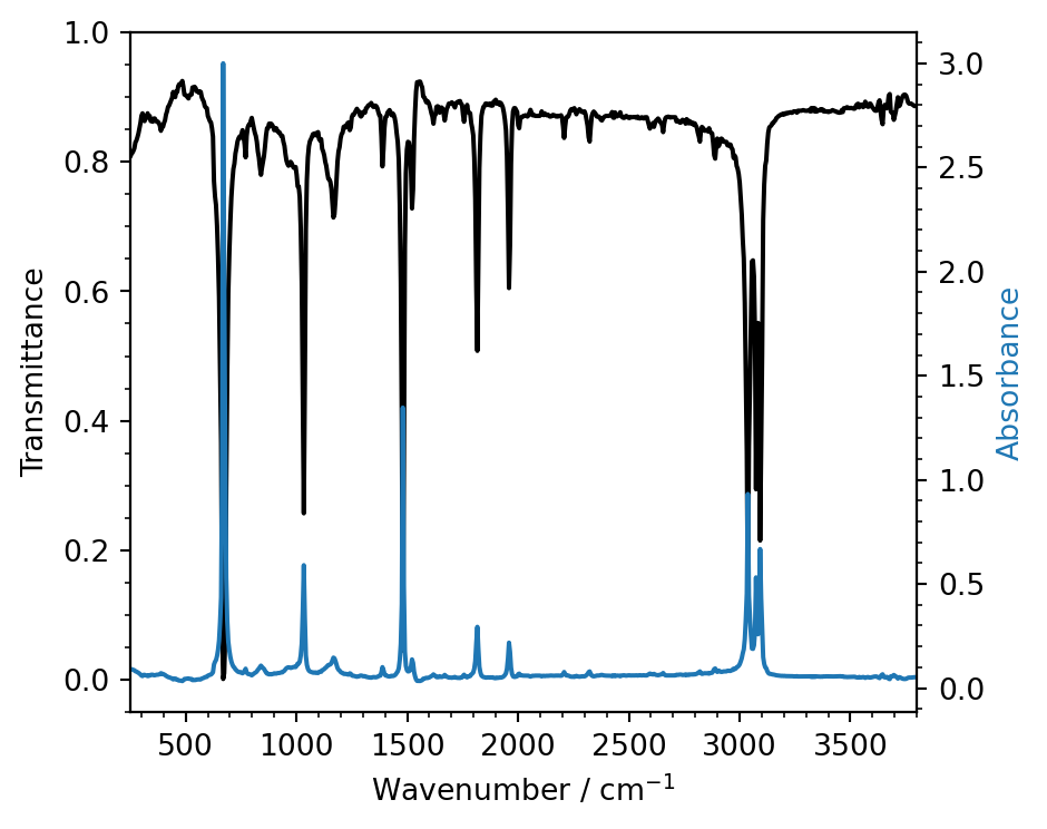
# Load the infrared data from filewavenumber, transmittance, absorbance = np.loadtxt('water_ir_spectrum.dat', unpack=True, skiprows=1)# Create the figure and the axesfig, ax = plt.subplots(figsize=(5, 4))ax.plot(wavenumber, transmittance, color='k', label='Transmittance')ax.set_xlabel(r'Wavenumber / cm$^\mathregular{-1}$')ax.set_ylabel('Transmittance')# Set axis limits and enable minor ticksax.set_ylim(-0.05, 1)ax.set_xlim(250, 3800)ax.minorticks_on()# Create twinned axis for absorbance# Twinx means they will share the x axis but have different y scalesaax = ax.twinx()# Plot absorbance data onto new twinned axisaax.plot(wavenumber, absorbance, color='C0', label='Absorbance')# Set y label for twinned axis with same color as the lineaax.set_ylabel('Absorbance', fontdict={'color': 'C0'})# Add minor ticksaax.minorticks_on()fig.tight_layout()plt.show()
Legends - contents and position
A figure legend should simply state which “thing” a given line corresponds to.
You should be able to use the axis labels and legend to read out the following sentence
This figure shows y_label as a function of/versus x_label for legend_entry_1, legend_entry_2, .. and legend_entry_n.
For example
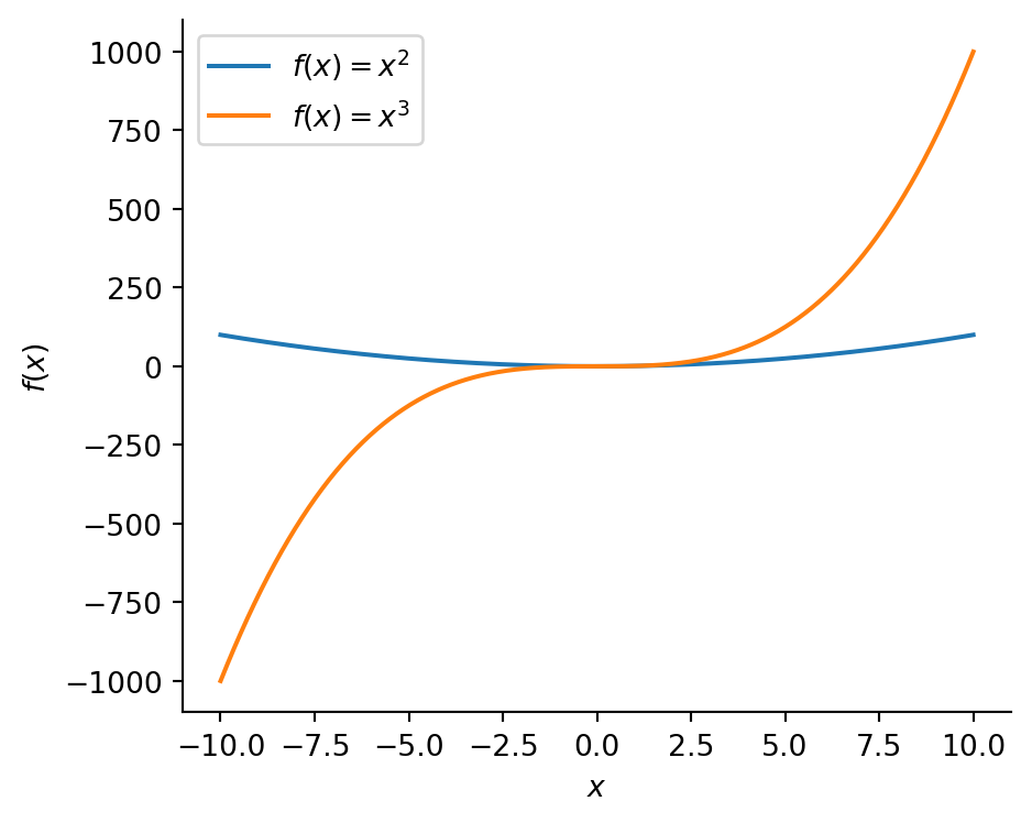
from matplotlib.ticker import MultipleLocator# 1000 linearly spaced values between -10 and 10x = np.linspace(-10, 10, 1000)# Create the figure and the axesfig, ax = plt.subplots(figsize=(5, 4))# Plot the data, and provide a label for each plot with custom coloursax.plot(x, x **2, label=r'$f(x) = x^2$')ax.plot(x, x **3, label=r'$f(x) = x^3$')# Remove right and upper spines# these are the "outlines" of the axisax.spines['top'].set_visible(False)ax.spines['right'].set_visible(False)# Set the axis labelsax.set_xlabel(r'$x$')ax.set_ylabel(r'$f(x)$')# Turn on the legendax.legend()# Tighten the layoutfig.tight_layout()# Show the plotplt.show()
“This figure shows \(f(x)\) versus \(x\) for \(f(x)=x^2\), and \(f(x)=x^3\).”
Or, another example is
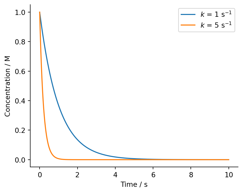
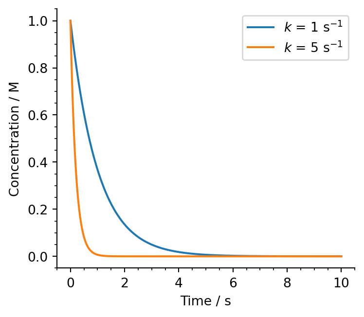
from matplotlib.ticker import MultipleLocator# Time values 0 to 10 secondst = np.linspace(0, 10, 1000)# 1st order rate constantsk1 =1# s^{-1}k2 =5# s^{-1}# Initial concentrationc0 =1# M# Concentrations as fn of time for two rate constantsconc_1 = c0 * np.exp(-k1 * t) # Mconc_2 = c0 * np.exp(-k2 * t) # M# Create the figure and the axesfig, ax = plt.subplots(figsize=(5, 4))# Plot the data, and provide a label for each plot with custom coloursax.plot(t, conc_1, label=r'$k$ = 1 s$^\mathregular{-1}$')ax.plot(t, conc_2, label=r'$k$ = 5 s$^\mathregular{-1}$')# Remove right and upper spines# these are the "outlines" of the axisax.spines['top'].set_visible(False)ax.spines['right'].set_visible(False)# Set the axis labelsax.set_xlabel(r'Time / s')ax.set_ylabel(r'Concentration / M')# Turn on the legendax.legend()# Tighten the layoutfig.tight_layout()# Show the plotplt.show()
“This figure shows concentration versus time for a first order reaction with \(k=1\, \mathrm{s^{-1}}\) and \(k=5\, \mathrm{s^{-1}}\).”
Your legend labels should not be anything like “concentration versus time” - this is what the axis labels are for.
Figure resolution
Use %config InlineBackend.figure_format='retina' once per notebook - this displays figures in high resolution.
When saving figures, ensure that you save them at a sufficiently high resolution, also known as DPI (dots-per-inch).
For word processed documents, dpi=300 will be sufficient, but this is more complex for presentations - see below.
Exporting your figure to Word or Powerpoint
You’ll certainly want to include your figure(s) in a Word processed document (e.g. in Microsoft Word), or a presentation (e.g. Microsoft Powerpoint).
As we’ve mentioned, in the past you’ll have manually scaled the figure inside of Word or Powerpoint, but this usually distorts your figure and makes it look, frankly, bad.
Word Processors (Microsoft Word)
When making a document in a Word processor, you always know the size of the document you’re producing. More often than not, you’ll be working with an A4 sized document. For the rest of this tutorial we’ll assume that’s the case, but if you’re working with something different then the approach below can be adapted.
The maximum width of a figure in Microsoft Word’s default (portrait) page width is 6.5 inches, so your figure should never be wider than this. A good figure width is 4 inches, so lets repeat our figure of \(x^2\) and \(x^3\) from earlier at this size.
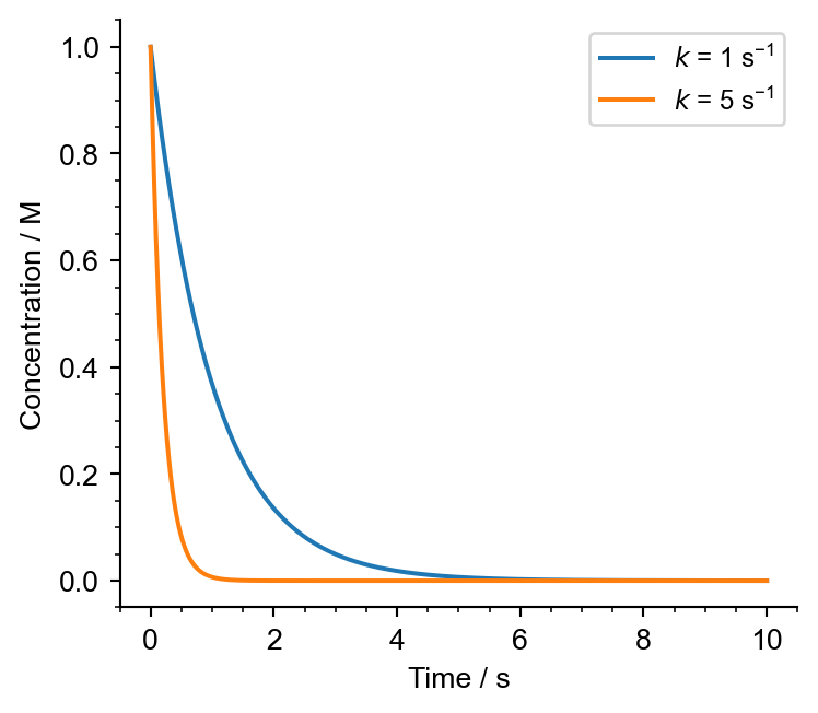
width =4# inchesheight =7/8* width# Create the figure and the axesfig, ax = plt.subplots(figsize=(width, height))# Plot the data, and provide a label for each plot with custom coloursax.plot(t, conc_1, label=r'$k$ = 1 s$^\mathregular{-1}$')ax.plot(t, conc_2, label=r'$k$ = 5 s$^\mathregular{-1}$')# Remove right and upper spines# these are the "outlines" of the axisax.spines['top'].set_visible(False)ax.spines['right'].set_visible(False)# Set the axis labelsax.set_xlabel(r'Time / s')ax.set_ylabel(r'Concentration / M')# Enable minor ticksax.minorticks_on()# Turn on the legendax.legend()# Tighten the layoutfig.tight_layout()# Show the plotplt.show()
We’ve made the height ever so slightly smaller than the width - this accounts for the room taken up by the \(y\) axis label, and keeps the actual plot roughly square.
The next thing we need to think about is the font size for our figure. We want this to be a little bit smaller than our document text (size 12), so we can choose size 10 for everything other than the legend which we’ll set to size 9. We’re also going to change the font family used in our plot to Arial, since this is what we’re using in our report. To do this you’ll need to upload this file to Noteable.
We can set all of these options by redefining Matplotlib's defaults. This only needs to be done once per notebook - every figure after this will use the new settings.
Remember that the DPI of an image states how many pixels (“dots”) are contained in a given inch.
For an image with a fixed size, higher DPI leads to a sharper image.
#### Font settings - these things only need to be configured once per notebook# Register Arial font import matplotlib.font_manager as fmfm.fontManager.addfont("Arial.ttf")# Set font size to 10, and legend font size to 9plt.rcParams['font.family'] ='Arial'plt.rcParams['font.size'] =10plt.rcParams['legend.fontsize'] =9##### Create the figure and the axesfig, ax = plt.subplots(figsize=(4, 3.5))# Plot the data, and provide a label for each plot with custom coloursax.plot(t, conc_1, label=r'$k$ = 1 s$^\mathregular{-1}$')ax.plot(t, conc_2, label=r'$k$ = 5 s$^\mathregular{-1}$')# Remove right and upper spines# these are the "outlines" of the axisax.spines['top'].set_visible(False)ax.spines['right'].set_visible(False)# Set the axis labelsax.set_xlabel(r'Time / s')ax.set_ylabel(r'Concentration / M')# Enable minor ticksax.minorticks_on()# Turn on the legendax.legend()# Tighten the layoutfig.tight_layout()# Save to fileplt.savefig('conc_report.png', dpi=300)# Show the plotplt.show()
Where we’ve also saved our plot to conc_report.png. We can now import this file into Word and set its width to 4 inches (or 10.16 cm) using the Picture Format tab. The result should look something like this.
Powerpoint
The situation for a Powerpoint presentation is a little bit different - you don’t (generally) know how big your slide will be when it appears on a projector, and so instead of working with distances like inches or centimetres, we have to work in units of pixels (the tiny squares that make up the image on your screen) since, although they change size between displays, the number of pixels is roughly constant. For example, compare a 4K 52 inch TV to a 4K projector: both have the same number of pixels (since they’re both 4K), but the pixels have different physical dimensions.
The full width of a slide will usually be between 1400 and 1600 pixels (for a modern 16:9 projector, and excluding margins), so we can use this information to size our plots accordingly.
To get Matplotlib to produce an image with a specified size in pixels we have to state the size of the image in inches, and the DPI of the image. This is slightly annoying, but these values can be obtained quite easily. For a Powerpoint slide, you can always set the DPI to 150 since, as we’re working in pixels, this will no longer affect the sharpness of the image in the same way as it did before (e.g. for a Word document).
To calculate the width in inches, we use the following simple formula
As an example, let’s make our concentration versus time graph 850 pixels wide. If we set our DPI as 150, then the width of the figure can be calculated.
# Calculate the figure size for a fixed number of pixels and dpipixels =850dpi =150width_in = pixels / dpiheight_in = width_in *7/8
Where we’ve selected a slightly smaller height than width so that we end up with a square plot, just as we did for a Word processed document.
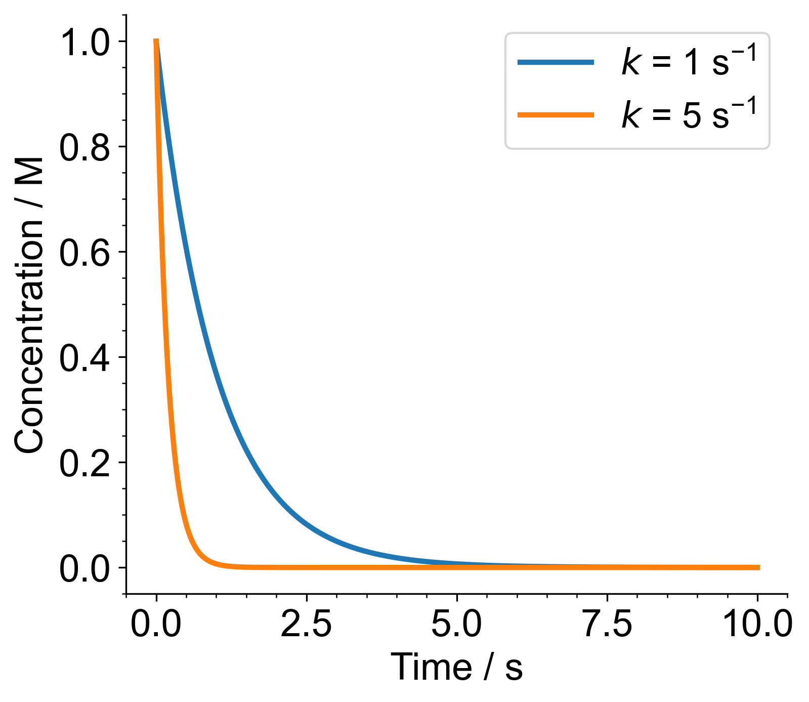
# Set font size to 18, and legend font size to 17plt.rcParams['font.size'] =18plt.rcParams['legend.fontsize'] =17fig, ax = plt.subplots(figsize=(width_in, height_in), dpi=dpi)# Plot the data, and provide a label for each plot with custom colours# Here we've used a thicker linewidth for our presentationax.plot(t, conc_1, label=r'$k$ = 1 s$^\mathregular{-1}$', lw=2.5)ax.plot(t, conc_2, label=r'$k$ = 5 s$^\mathregular{-1}$', lw=2.5)# Remove right and upper spines# these are the "outlines" of the axisax.spines['top'].set_visible(False)ax.spines['right'].set_visible(False)# Set the axis labelsax.set_xlabel(r'Time / s')ax.set_ylabel(r'Concentration / M')# Enable minor ticksax.minorticks_on()# Turn on the legendax.legend()# Tighten the layoutfig.tight_layout()# Save to file but no need to specify DPI - the value# used in plt.subplots will be used.plt.savefig('conc_pres.png')# Show the plotplt.show()
This looks like a huge plot when viewed on this website, and on Noteable! But, if imported into Powerpoint and set with a width of 850 px in the Picture Format tab, you’ll get a slide that looks like this.
One last thing - font sizes. The projector image is definitely going to be bigger than A4, so we’re going to need a larger font size than 12.
The following are recommended font sizes for slides:
Slide Element
Recommended Font Size (for Arial)
Title
32–40 pt
Section header
26–32 pt
Main body text
20–24 pt
Figure text
18–22 pt
Figure captions
16–18 pt
Footnotes / References
14–16 pt (minimum)
A good choice is a figure text size of 18, and a legend text size of 17 - this is what we’ve used in the example above. Notice that when the above procedure is followed, the font size on the image is correct versus that of a text box with equivalently sized text.